


When a project has several possible risk responses, a decision tree helps you compare the choices and the uncertain events that may follow. It shows the available actions, their possible outcomes, the probabilities you assign to those outcomes, and the consequences you need to consider.
This guide explains the structure, shows how to organize it in Boardmix, and works through a release decision using expected monetary value. The calculation makes assumptions easier to discuss; it does not remove uncertainty or decide which losses your team can afford.
What is decision tree analysis?
Decision tree analysis is a visual method for comparing alternatives under uncertainty. Starting at a choice, you follow branches through possible events to their outcomes. You then work backward to evaluate the alternatives using a consistent measure, such as net monetary value or total cost.
This decision-analysis tree differs from a machine-learning decision tree, which is trained on data to make predictions. In a project risk model, the decision maker supplies the alternatives, probability estimates, and outcome values.
The Project Management Institute's discussion of quantitative decision methods connects decision trees with expected monetary value, or EMV: multiply each possible net outcome by its probability, then add the results.
The role of decision tree analysis in project risk
A tree can clarify which risk response is worth investigating and which assumptions drive the comparison. Its practical uses include:
- Showing the alternatives: keep the actions, uncertain events, and consequences visible in one model.
- Structuring a complex choice: break a decision into branches that can be assessed separately.
- Making estimates explicit: attach a source or rationale to probabilities and costs so others can challenge them.
- Comparing scenarios: change an uncertain input and examine whether the preferred option changes.
A diagram cannot make weak data reliable. If the team has not identified the risks yet, a project premortem can help uncover plausible failure scenarios before you estimate their probabilities.
Elements and structure of a decision tree
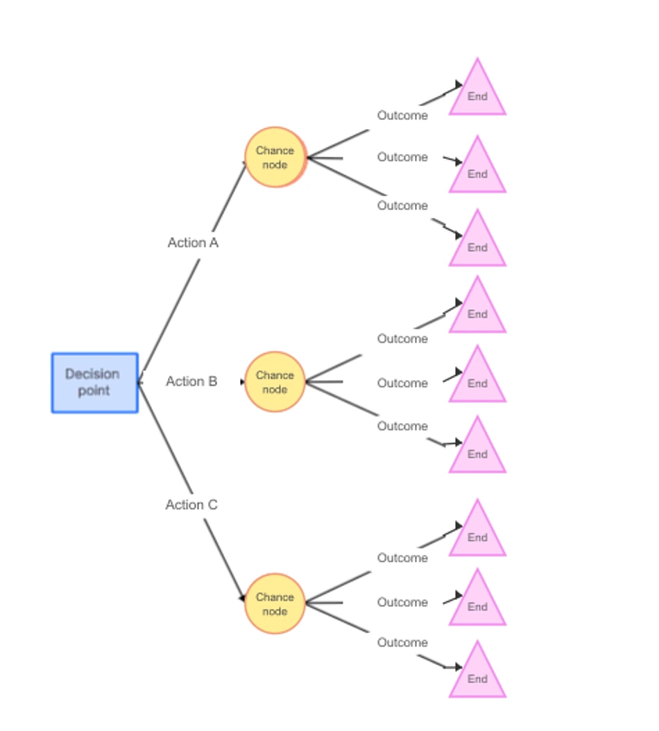
| Element | Meaning | Example label |
|---|---|---|
| Decision node, usually a square | A choice under your control | Test first or release directly |
| Chance node, usually a circle | An uncertain event | No serious issue or serious issue |
| Branch | An action or possible event | Action name, or event and probability |
| Terminal node | The end of a modeled path | Net payoff or total cost |
Read the tree from left to right to follow a possible path. Outcomes leaving a chance node must be mutually exclusive and cover the possibilities in that part of the model. Their probabilities must sum to 1. Probabilities at later chance nodes are conditional on reaching those nodes.
How to draw the analysis in Boardmix
1. Start with a template or a blank canvas
Use the online decision tree template as a starting layout, or open Boardmix and create a board. State the decision at the left: “Test before release or release directly?” A clear question keeps unrelated uncertainties out of the diagram.
2. Add the choices, events, and outcomes
Use shapes and connectors to draw the branches. Put the probability on an event branch and the net payoff or cost at its endpoint. Short notes beside the diagram can explain the period being considered and the source of an estimate.
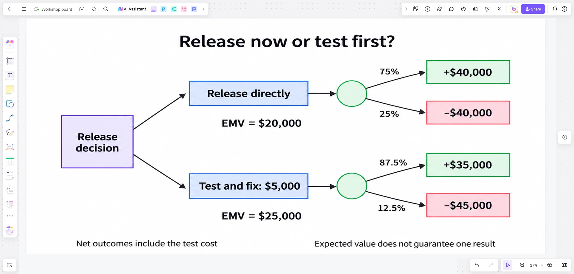
For the release example below, add two action branches. Each leads to a chance node with “No serious issue” and “Serious issue” outcomes. Keep the test cost visible and apply it consistently to both outcomes on the testing branch.
3. Evaluate and annotate the model
Calculate EMV with a calculator or spreadsheet if needed, then add the evaluated values beside the nodes. The whiteboard helps people discuss the model; drawing a tree does not itself verify the arithmetic. Keep alternatives that fail mandatory quality or safety requirements out of the feasible set, even if their calculated payoff looks attractive.
Four principles for a useful decision-tree analysis
1. Define the objective and the available options
List the alternatives at each decision point and identify the constraint you are trying to manage. “Reduce expected loss” is different from “avoid any loss above our available reserve.” Use the objective to decide which consequences the model must include.
2. Estimate the outcomes and their probabilities
Use relevant project information, test results, or comparable experience where available. Record what remains uncertain. Avoid adding a precise percentage simply because the diagram has a space for one.
3. Evaluate outcomes on a consistent basis
Do not mix gross revenue on one path with net profit on another. Specify whether costs have already been deducted from terminal values. For nonfinancial consequences such as customer disruption, keep an explicit note rather than inventing a dollar value to complete the calculation.
4. Interpret the result and choose a response
The highest EMV is the highest average monetary outcome under the model's assumptions, not automatically the best decision. PMI's analysis of risk-averse decisions explains why an organization may place more weight on avoiding an unaffordable loss than on maximizing an average payoff.
Worked example: test before release or release directly?
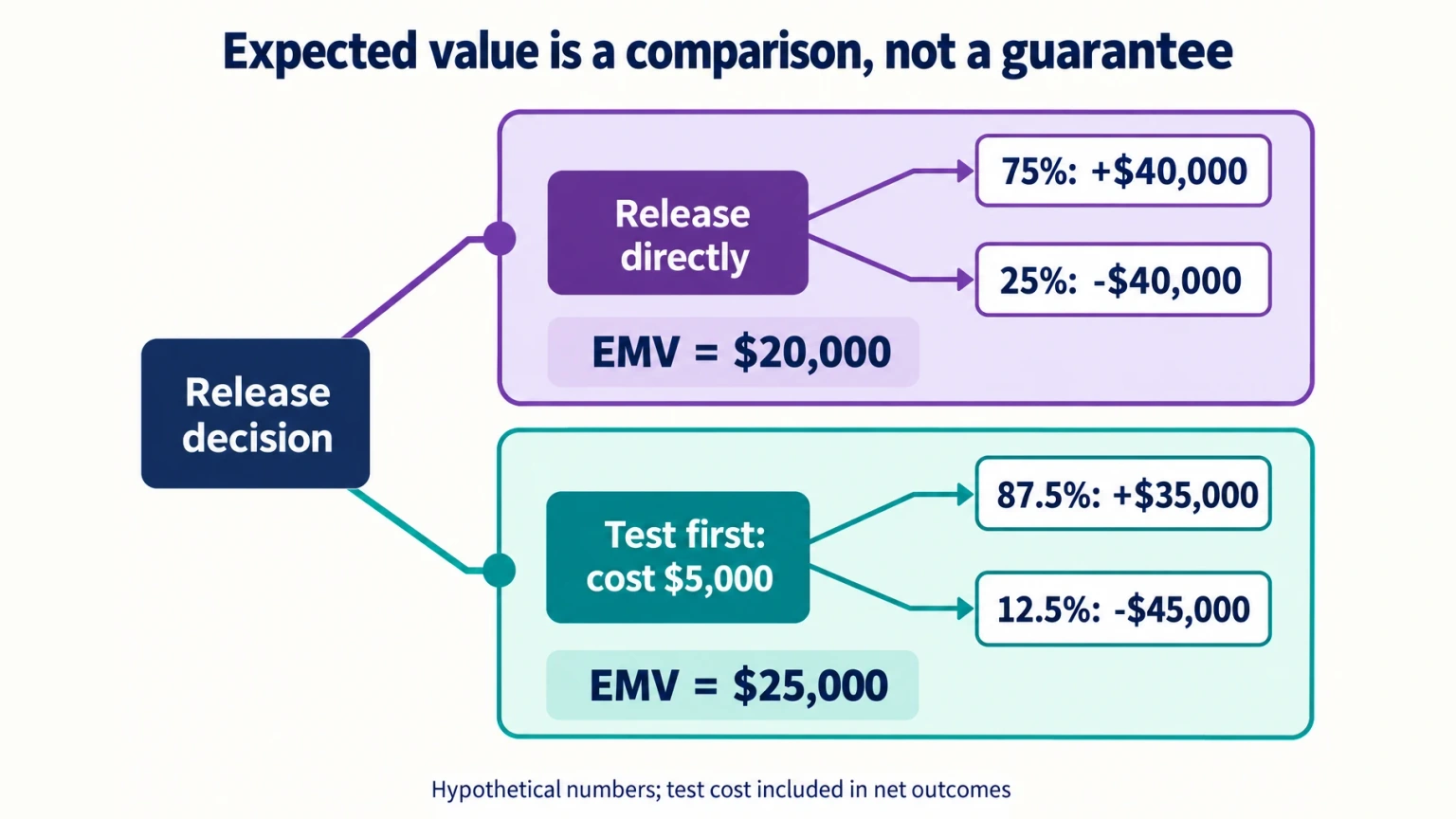
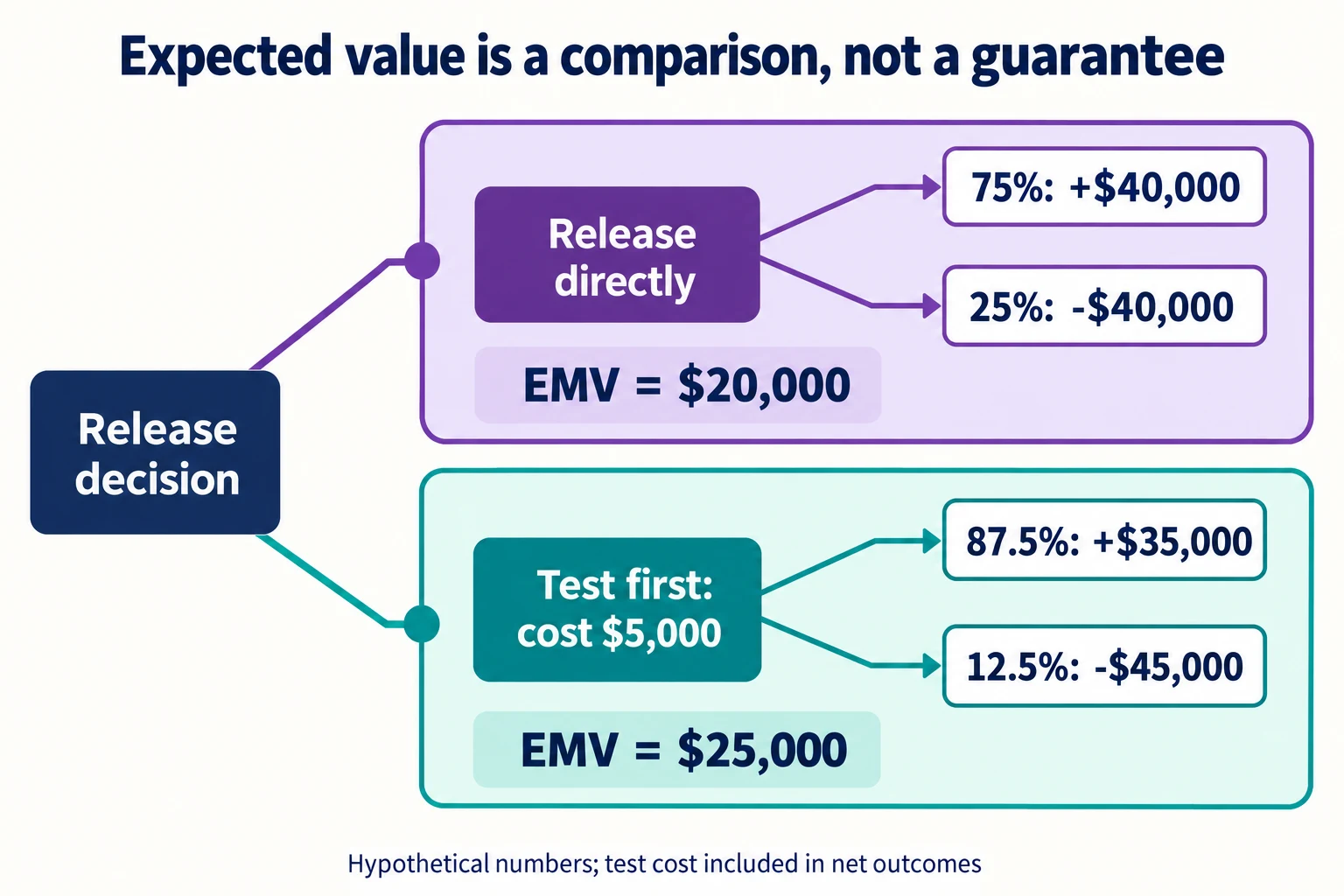
Suppose a team can release a feature directly or pay for additional testing and fixes. These are hypothetical teaching assumptions: a release without a serious issue produces $40,000 in net value before the additional testing cost; a release with a serious issue produces −$40,000. Direct release has a 25% issue probability.
The test-and-fix option costs $5,000 and is assumed to reduce the remaining issue probability to 12.5%. Its terminal payoffs are therefore $35,000 and −$45,000. Testing alone does not imply that reduction; the assumption includes fixing the issues found.
| Option | No serious issue | Serious issue | EMV |
|---|---|---|---|
| Release directly | 0.75 × $40,000 | 0.25 × −$40,000 | $20,000 |
| Test first | 0.875 × $35,000 | 0.125 × −$45,000 | $25,000 |
Direct release: $30,000 − $10,000 = $20,000. Testing: $30,625 − $5,625 = $25,000. Subtracting the $5,000 test cost again would count it twice.
Testing has a $5,000 EMV advantage under these assumptions. Its worst outcome is still worse: −$45,000 rather than −$40,000. The team needs to consider whether it can absorb that loss and whether the estimated improvement is credible.
Which assumption could reverse the decision?
If q is the remaining issue probability after testing, the testing option's EMV is $35,000 − $80,000q. Equating this to the direct-release EMV gives:
$35,000 − $80,000q = $20,000; q = 18.75%.
Testing wins on EMV below 18.75%, while direct release wins above that threshold, with the other assumptions unchanged. At 20%, testing's EMV is $19,000; at 10%, it is $27,000. This focuses the next discussion on the evidence for reducing the issue probability.
For a diagram without monetary calculations, the general decision tree guide explains the basic structure. For this risk model, create the decision tree in Boardmix and keep the choices, assumptions, and sensitivity result together so reviewers can discuss the input that drives the decision.